The Chow-Robbins game with an unknown coin
12 Nov 2018The Chow-Robbins game is a classic example of an optimal stopping problem. It was introduced by Yuan Shih Chow and Herbert Robbins [1] who proved existence of the optimal policy and the value function for this problem. Inspired by their work, Aryeh Dvoretzky [2] presented an asymptotic bound on the optimal number of heads after $n$ coin tosses. Several years later, Larry Shepp [3] found the exact constant in that bound, which showed that the proportion of heads required for stopping after $n$ coin tosses is asymptotically equal to \begin{equation} \frac{1}{2} + \frac{0.41996\dots}{\sqrt{n}}. \end{equation} Unfortunately, this asymptotic result says nothing about the optimal policy in the beginning of the game. Only recently, rigorous computer analysis has been carried out by several authors [4,5,6]. Their calculations provided high-precision numerical estimates of the payoff together with useful bounds and explicit tables describing the optimal policy.
Although there is no straightforward description of the optimal policy rather than through an infinite sequence of numbers, Jon Lu [7] analysed several suboptimal policies and showed that a simple-minded rule that can be described as stop when the number of heads first exceeds the number of tails already delivers the expected payoff of $\pi/4 \approx 0.7854$, which is within $1\%$ from the optimum—remarkably close. This renewed interest in the Chow-Robbins game led to an extension of the problem to a setting with a biased coin presented by Arjun Mithal [8] earlier this year. In this post, we take it one step further and drop the assumption that the bias of the coin is known in advance but rather let the player discover it over time. Somewhat surprisingly, numerical simulations show that the Bayes-optimal coin-agnostic policy under a flat prior on the coin bias is for all practical purposes identical with the optimal fair-coin policy.
Dynamic programming solution
Let $b_1, b_2, \dots$ be a sequence of i.i.d. Bernoulli random variables with bias $\theta$, i.e., the probability of heads is $P(b_i = 1) = \theta$. Denote partial sums of this series by $s_t = b_1 + \dots + b_t$. The dynamics of this sum can be written as \begin{equation} s_t = s_{t-1} + b_t,\quad s_0 = 0,\quad t=1, 2, \dots \label{dynamics} \end{equation} The expected payoff is given by $E[s_t/t]$ where $t$ is a stopping time. The objective is to find a stopping time that maximizes the expected payoff.
We assume that the player does not know $\theta$ in advance. Therefore, we put a uniform prior over the interval $[0, 1]$. After $t$ coin tosses, the state of the game is fully described by the tuple $(t, s_t)$ containing the total number of coin tosses $t \in \{1, 2, \dots\}$ together with the number of heads so far $s_t \in \{1, 2, \dots, t\}$. The posterior over the coin bias $\theta$ after $t$ coin tosses is given by the Beta distribution \begin{equation} p(\theta | t, s_t) \propto \theta^{s_t} (1 - \theta)^{t - s_t}. \label{posterior} \end{equation} The Bellman equation for this problem can be written as \begin{equation} v_t(s_t) = \max \left\{ \frac{s_t}{t}, E\left[v_{t+1}(s_{t+1}) | t, s_t \right] \right\}. \label{dp} \end{equation} It says that after $t$ coin tosses, the player compares what he has got so far, $s_t/t$, with what he expects to make in the future, $E\left[v_{t+1}(s_{t+1}) | t, s_t \right]$, and whichever is greater he calls the value of the current state $(t, s_t)$. Assuming $v_t(s_t)$ exists for all states $(t, s_t)$ and is known to the player, the optimal policy is very simple: the player should stop as soon as $s_t/t \geq E\left[v_{t+1}(s_{t+1}) | t, s_t \right]$ for the first time.
Despite knowing that $v_t(s_t)$ exists—thanks to Chow and Robbins [1]—computing it is not straightforward because the base of induction \eqref{dp} lies at infinity; this is an example of a free boundary problem [11]. What we can do, however, is to cut the horizon, requiring all games to terminate by time $T < \infty$. Then the value of any state beyond the horizon is zero, i.e., $t > T \Rightarrow v_t(s_t) = 0$, and we can run the backward induction \eqref{dp} to find the value function at all times $1 \leq t \leq T$.
The last step before delving into implementation details is to expand the expectation in \eqref{dp} using the system dynamics \eqref{dynamics} and the posterior \eqref{posterior}. We can do it as follows
Thus, we simply need to iterate the following scheme \begin{equation} v_t(s_t) = \max \left\{ \frac{s_t}{t}, \frac{t-s_t+1}{t+2} v_{t+1}(s_t) + \frac{s_t+1}{t+2} v_{t+1} (s_t+1) \right\}. \label{explicit_dyn_prog} \end{equation} One peculiar property of \eqref{explicit_dyn_prog} is that the size of the state variable $s_t$ depends on the other state variable $t$; namely, $s_t \in \{1, 2, \dots, t\}$. Apart from that, it is a usual value iteration scheme. The expected payoff of the game is then given by \begin{equation} v_0(0) = \frac{1}{2}v_1(0) + \frac{1}{2} \end{equation} where we already substituted $v_1(1) = 1$ because the optimal policy for any coin is to stop after the first toss if it turned out heads.
Numerical analysis
We present two plots which give some food for thought. It is in no sense a comprehensive analysis but it gives a taste for the difficulties one is facing when approaching this problem. The code for generating the plots can be found here.
Classic Chow-Robbins game
First, we consider the classic Chow-Robbins game with a known fair coin. In this case, we should set both coefficients in front of the value function on the right-hand side of \eqref{explicit_dyn_prog} to $1/2$ to obtain the correct value iteration algorithm.
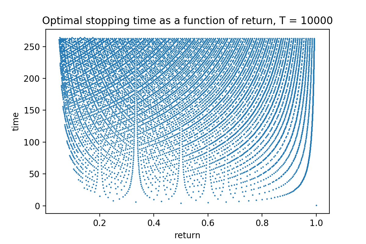
For any value of the return, there is a time point at which it is optimal to stop the game. This plot shows the non-trivial dependence between the optimal stopping time and the return.
The figure above depicts the function: $\textrm{return} \mapsto \textrm{stopping time}$ for which this return is optimal. It is not a one-to-one function because it may be optimal to stop at a certain time for two different values of return. This claim is true for a finite-horizon problem (e.g., $T = 10000$ in the figure above). Since this approximation is quite good and not much changes if one increases $T$ even by a factor of $10$, I would expect that it also holds for the infinite-horizon problem, but it would be nice to have a rigorous proof of that statement.
Specificity vs universality
Second, we study the effect of not knowing the coin in advance. For this purpose, we conduct two experiments. In one experiment, we compute the value function for a specific coin and then evaluate the policy derived from that value function on a range of possible coins. This experiment is repeated on several coins. In the second experiment, we compute the value function which is independent of the coin and then evaluate the corresponding policy on other coins.
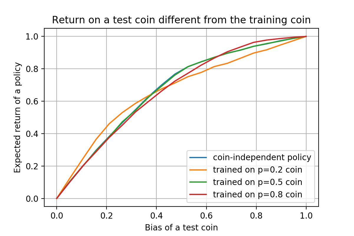
Expected return of a given policy depends on the coin used for policy evaluation. Surprisingly, the coin-independent policy (blue line) and the fair-coin policy (green line) coincide. On the other hand, coin-specific policies (e.g., orange and red lines) perform better on the coins close to the one for which they were designed but perform worse on other coins, as expected.
Numerical simulations, results of which are depicted in the figure above, show that assuming that the coin is unknown and learning about its parameters through experimentation performs as good as assuming that the coin is fair and just going with it. On the other hand, if the bias of the coin is known, then the optimal policy for that specific coin beats both the fair-coin policy as well as the coin-independent policy, as one would expect. Somewhat surprisingly, however, the area under the curves is almost the same for all curves. It is surprising because the area represents the expected return of a policy over a uniform distribution of coin biases; since the coin-independent policy is specifically designed to optimize exactly this criterion, one would expect it to beat coin-specific policies—and indeed it does, but the difference is only slightly above $1\%$.
Conclusion
We only scratched the surface of a very simple optimal stopping problem. If you want to learn more about optimal stopping and applications, check out the book by Thomas S. Ferguson [9] for an overview. A slightly older but very enjoyable overview paper was written by maestro Robbins himself [10]. For connections between optimal stopping and free boundary problems, see the deep and insightful paper by Pierre van Moerbeke [11].
The elusive beauty and elegance of the value function of the Chow-Robbins game captivated imagination of Samuele Tosatto and me over a few coffee breaks. Later we discovered that this problem attracted many great minds [12]. Although we were not able to find a closed-form solution, we were pleased to find out that solving a seemingly more complex problem (when the coin is unknown) is actually not harder than solving the original one, at least as far as numerical computation is concerned. On the downside, not knowing the coin bias seems to be as good as assuming the coin is fair. Nevertheless, it would be nice to prove the existence of the value function in the infinite-horizon case.
Bibliography
- Yuan Shih Chow and Herbert Robbins, On optimal stopping rules for $s_n/n$, Illinois J. Math., 9(3):444-454, 1965.
- Aryeh Dvoretzky, Existence and properties of certain optimal stopping rules, Proc. Fifth Berkeley Symp. on Math. Stat, and Prob., 1:441-452, 1965.
- Larry A. Shepp, Explicit solutions to some problems of optimal stopping, The Annals of Mathematical Statistics, 40:993–1010, 1969.
- Julian D. A. Wiseman, The expected value of $s_n/n \approx 0.79295350640\dots$ http://www.jdawiseman.com/papers/easymath/coin-stopping.html, 2005.
- Luis A. Medina and Doron Zeilberger, An Experimental Mathematics Perspective on the Old, and still Open, Question of When To Stop? Gems in Experimental Mathematics, 517:265-274, 2010.
- Olle Häggström and Johan Wästlund, Rigorous Computer Analysis of the Chow–Robbins Game, The American Mathematical Monthly, 120(10):893-900, 2013.
- Jon Lu, Analysis of the Chow-Robbins game, https://math.mit.edu/~apost/courses/18.204-2016/, 2016.
- Arjun Mithal, Analysis of the Chow-Robbins Game with Biased Coins, https://math.mit.edu/~apost/courses/18.204_2018/, 2018.
- Thomas S. Ferguson, Optimal Stopping and Applications, http://www.math.ucla.edu/~tom/Stopping/Contents.html, 2008.
- Herbert Robbins, Optimal Stopping, The American Mathematical Monthly, 77(4):333-43, 1970.
- Pierre van Moerbeke, Optimal stopping and free boundary problems, The Rocky Mountain Journal of Mathematics, 4(3):539-578, 1974.
- Zhiliang Ying and Cun-Hui Zhang, A Conversation with Yuan Shih Chow, Statist. Sci., 21(1):99-112, 2006.